Linear Regression

Linear Regression is a topic long studied in statistics and recently it has been widely used in machine learning models. Because of its its simplicity and efficiency, in some applications it is considered a good practice to test new models with linear regression before attempting more sophisticated algorithms.

Gaining intuition

Imagine we have information about the number of people that visited a given store in São Paulo and the total sales at that store in 9 different months. Imagine the information is as follows:

If the owner of that store wanted to estimate the number of sales on a given month based on the number of people that visited the store, one strategy would be to use a 'trendline' to estimate the sales. A trendline is line that captures the "trend" in the data, that is, a line that approximates the data. One example is given bellow:

With that line the owner of the store can predict that if 20 people visit the store, the sales will be around $1000, and if 120 people visit the store, the sales will be around $5050.

The challenge we face is that many lines can be said to approximate the data above. How can we chose the best one? As with any approximation, the line we choose will lead to errors. A natural idea is to choose the line that minimizes the sum of the errors in each point. That is precisely what we will do.

We can measure the error we make in a given estimation by taking the difference from our prediction (a point on the line) to the point in the dataset. That will give us the error we make at each point. Our model, for instance, tells us that if 100 people visit the store, the sales will be around $4100, while the data shows that sales were of $5500. The error we made with that estimate was of $1400. To get the total error we sum the errors at each point.

Since some points are above the line and some are bellow, we would have positive and negative numbers that could cancel out. To prevent that, a good strategy is to take the square of theses differences. Taking that into account, we can say the total error we make with a given line is \(\sum_{i=1}^n (f(x_i) - y_i)^2 \), where \(y_i\) is the y-coordinate of the data-point and \(f(x_i)\) is our prediction. We will consider the best line, the one that reduces this error. This strategy is called least squares. When using this strategy it is computationally useful to divide the whole equation by N, the number of data-points we are considering. This then becomes the "mean squared error", and we avoid operations with big numbers.

$$E = \frac{1}{N} \sum_{i=0}^n \left( f(x_i) - y_i \right)^2$$

The line we get by minimizing this error function is our linear-regression line.

Analytical Solution

In the example above, the function f can be represented by a line, but real-world applications often involve way more than two dimensions. The total sales from a given store, for instance, is not only a function of the number of people that visited the store - there are many other variables to take into account. Let's see how we can find a linear function that minimizes the error in a more general scenario.

The line of best-fit in the example we saw, can be modeled as \(y = f(x) = w_1x + w_0 \), where \(w_0\) and \(w_1\) are constants. The task of finding the best-fit line can be rephrased to finding \(w_0\) and \(w_1\) that minimize the error function. If we had more variables, our best-fit function would look like \(y = f(x) = w_nx_n + w_{n-1}x_{n-1} \dots + w_0 \), where \(w_i\) can be interpreted as the weight of the variables \(x_i\) in the prediction. In other words, \(w\) represents the influence of \(x_i\) in the prediction \( y \).

To simplify our notation it would be useful to rewrite this in the vector/matrix form as \(\bf{w}^Tx\), where \(\bf{w}\) is called the weight vector, and \(\bf{x}\) represents the observations we make. Notice, however that \(w\) has 1 dimensions more than \(x\), because of the constant \(w_0\). To deal with that, we will add 1 dimension to \(x\) and consider \(x_0 = 1\). Using this notation we can rewrite our error function as $$E(\bf{w}) = \frac{1}{N} \sum_{i=0}^n \left( \bf{w}^Tx_i - y_i \right)^2$$ To further simplify the math we will consider the vector of errors (scroll left to see the all the steps):

$$ \begin{bmatrix} \bf{w}^T x_1 - y_1 \\ \bf{w}^T x_2 - y_2\\ \dots \\ \bf{w}^T x_N - y_N\\ \end{bmatrix} = \begin{bmatrix} \bf{w}^T x_1 \\ \bf{w}^T x_2 \\ \dots \\ \bf{w}^T x_N \\ \end{bmatrix} - \begin{bmatrix} y_1\\ y_2 \\ \dots \\ y_N \\ \end{bmatrix} = \begin{bmatrix} \bf{w}^T x_1 \\ \bf{w}^T x_2 \\ \dots \\ \bf{w}^T x_N \\ \end{bmatrix} - y = \begin{bmatrix} w_0 + w_1x_{11} + \dots + w_d x_{1d} \\ w_0 + w_1x_{21} + \dots + w_d x_{2d} \\ \dots \\ w_0 + w_1x_{N1} + \dots + w_d x_{Nd} \\ \end{bmatrix} - y = \begin{bmatrix} 1 & x_{11} & \dots & x{1d}\\ 1 & x_{21} & \dots & x{2d}\\ & & \dots & \\ 1 & x_{N1} & \dots & x{Nd}\\ \end{bmatrix} \begin{bmatrix} w_0\\ w_1\\ \dots\\ w_n\\ \end{bmatrix} - y = \bf{Xw} - y $$

We can now represent our mean squared error as

$$E(\bf{w}) = || \bf{Xw} - y||^2$$

To minimize this function we can we solve the equation

$$\nabla E(w) = \frac{2}{N} (X)^T (Xw - y) = 0 $$

which results in

$$X^TXw = X^Ty$$

\(w = (X^TX)^{-1}X^Ty\)

With that, we have the function \(f(x) = \bf{w}^Tx\) that minimizes the error!

Iterative Solution

The solution we found above is called the analytical or closed-form solution. That give us exact values for the weights we wanted to calculate. That solution, however requires calculating a matrix inverse, which is computationally expensive (an operation of cubic order to be specific). That means that finding an analytical solution can be very time-consuming and even impossible for large enough vectors. Gladly, we can use another strategy called gradient descent to calculate the weights.

A powerful solution: The idea behind gradient descent

Gradient descent deserves its own blog post (hopefully coming soon!). It is a widely used technic in many machine learning algorithms. In this post however we will see a quick explanation and a direct application of gradient descent.

The gradient of a multivariable function calculated in a certain point is the vector that indicates the direction and the rate of fastest increase in the function value at that point. What we will do in gradient descent is to start a vector \(\bf{w_0}\) with random weights, and repeatedly update this vector in the direction opposite to the gradient vector of our error function. This means we will start a point \(\bf{w_0}\) and update it generating a sequence of \(\bf{w_i}\) in the direction of fastest decrease of the error function. Therefore, we will update \(\bf{w_i}\) in the direction that minimizes the error. That is precisely what we wanted!

This is a powerful idea because it can be applied to other error functions. In other models such as logistic regression, we will use the same principle!

Calculating Gradient descent

Back to our linear regression, let us calculate the gradient vector of our error function. The gradient vector is calculated as follows:

$$\nabla E(\bf{w}) = \left( \frac{\partial E}{\partial w_0}, \frac{\partial E}{\partial w_1},\dots ,\frac{\partial E}{\partial w_d} \right)$$

Remember our error function is \(E(\bf{w}) = \frac{1}{N} \sum_{i=0}^n \left( f(x_i) - y_i \right)^2 \), where \(f_i\) can also be represented as \(\bf{w}^Tx_i\). So each component \(j\) of the gradient can be calculated as

$$\begin{aligned} \frac{\partial E}{\partial w_j} &= \frac{\partial} {\partial w_j} \frac{1}{N} \sum_i (f(x_i) - y_i)^2\\ &= \frac{1}{N} \sum_i \frac{\partial} {\partial w_j} (f(x_i) - y_i)^2\\ &= \frac{1}{N} \sum_i 2(f(x_i) - y_i) \frac{\partial}{\partial w_j} (f(x_i) - y_i)\\ &= \frac{2}{N} \sum_i (f(x_i) - y_i) \frac{\partial}{\partial w_j} ((w_0 + w_1x_{i1} + \dots + w_dx_{id}) - y_i)\\ &= \frac{2}{N} \sum_i (f(x_i) - y_i)x_{ij}\\ &= \frac{2}{N} \sum_i (\bf{w}^Tx_i - y_i)x_{ij} \end{aligned}$$

With that, we can calculate the whole gradient vector in a matrix form with \(\nabla E(w) = \frac{2}{N} X^T (Xw - y)\). With that we calculate the updates to the weight vector with \(\Delta w = -\nabla E(w) = - \frac{2}{N} X^T (Xw - y)\).

The algorithm

Now that we know how to calculate the gradient vector we can apply the algorithm described above. First we calculate the gradient, then we update the weights in a direction opposite to the gradient.

Notice that for the purpose of minimizing the error function we are not interested in the length of the vector, only in its direction. That means we can disconsider the constant \(2\) multiplying the vector. We will instead multiply the whole vector by a small value \(\eta\), known as the learning rate. (More on that later!)

We also need to define when to stop the algorithm. For now we will choose a number of iterations (known as the number of epochs) and stop the algorithm when we reach that number of iterations.

The complete algorithm is described bellow, it uses numpy (np) and the matrix form of the equations above to simplify the code.

# Add a column of ones to X to account for the bias
X = np.insert(X, 0, 1, axis=1)

# Number of samples and dimensions
n_samples, d = X.shape

# Initialize weights
w = np.zeros(d)

# Define the number of iterations and the learning_rate
epochs = 10000
learning_rate = 0.01

# Gradient Descent
for _ in range(epochs):
# Predict the values (apply f(X))
    y_predicted = np.dot(X, w)
    
    # Compute the gradients
    dw = (1 / n_samples) * np.dot(X.T, (y_predicted - y))
    
    # Update weights
    w -= learning_rate * dw

                    

A few words on the learning rate and the number of epochs

In the section above we arbitrarily chose a learning rate and a number of epochs. In real world applications there are heuristics that help determine these values. In another blog post I plan to explore strategies to determine when to stop an iterative algorithm like gradient descent. For the learning rate in some cases, the best we can do is to try different values and choose the ones with the best results. But here is some intuition on what happens if the learning rate is to big or to small.

If the learning rate is to small, the algorithm will need many iterations to converge, that means more time training the algorithm (calculating the weights). But if the learning rate is to big, the algorithm might not converge! The following image might help to illustrate.

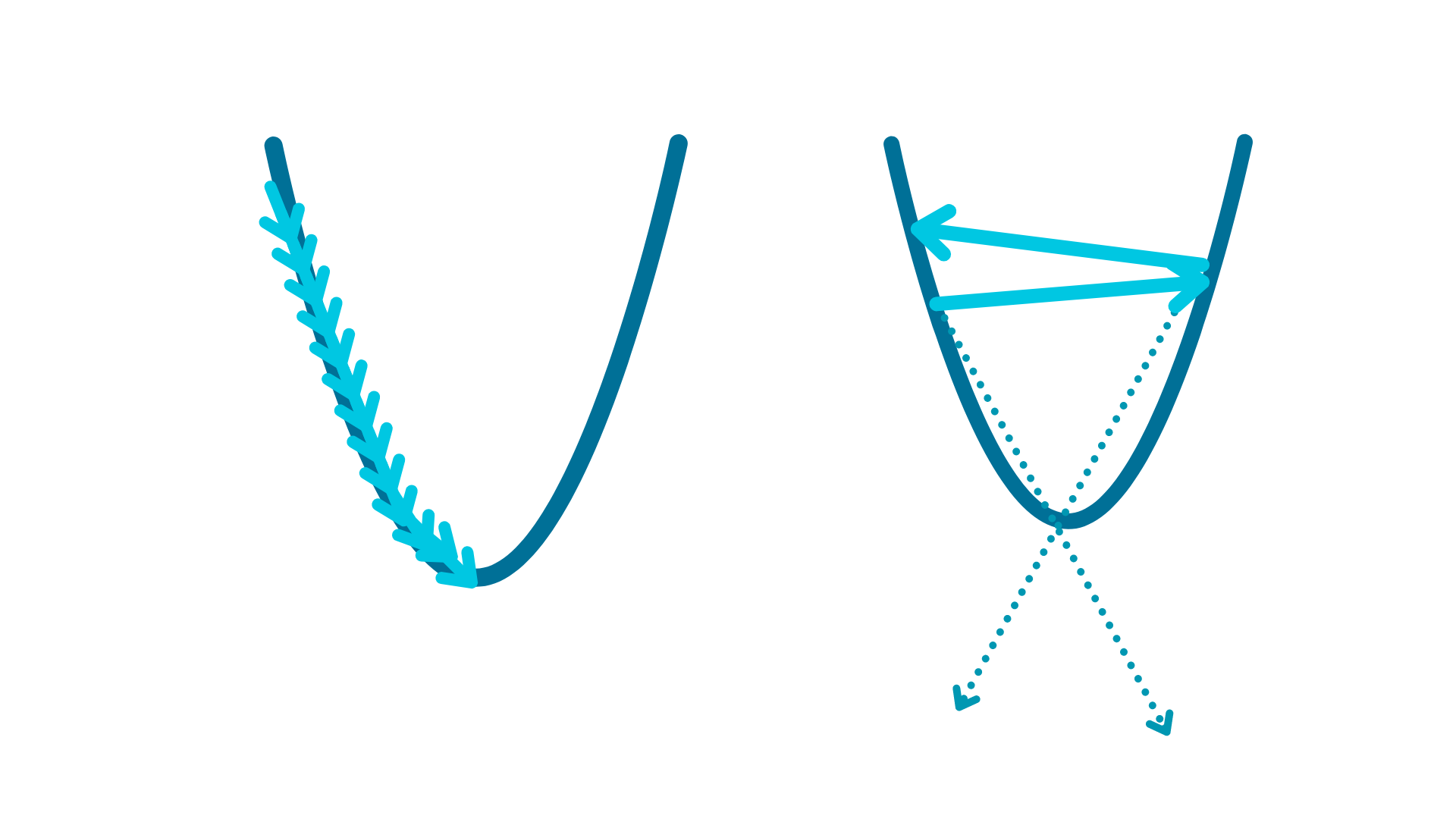
When the learning rate is too big the gradient is calculated in the right direction, but the algorithm might move far past the function minimum. This might lead the algorithm to never converge. Sometimes a good approach is to start with a big learning rate and to reduce it after some iterations. This might help to move fast toward the minimum, and increase the likelihood of convergence.

Conclusion

Linear Regression is a simple model and can be very useful in scenarios where the data can be modeled linearly. But even when the data is not linear, the ideas we saw here appear everywhere. In future posts we will see how to apply the ideas learned here to other models.