Introduction to Neural Networks - Part I

Neural Networks take advantage of simple building blocks to create powerful models for classification and regression problems. The goal of this post is to introduce Perceptrons and their components, preparing us for more complex Neural Network models.

Perceptrons - The Building Blocks

Perceptrons are a simple tool useful for binary classification problems. A classic example is the problem of approving or denying credit in a bank. We can collect data from individuals in a vector \(x \in \mathbf{R}^d\), which will be our input space, and represent our decision with \(Y = \{+1, -1\}\), our output space. The different coordinates in \(X\) correspond to information like salary, debt, age, and other fields. The goal of a perceptron is to classify new points in our input space as +1 or -1. The perceptron applies a function that weights each of the coordinates in the input, sums them up, and compares the result to a threshold. If the weighted sum of the input is above the threshold, we label the point as +1; if it is below the threshold, we label it -1.

This idea can be represented as $$h(x) = sign\left(\left( \sum^{d}_{i=0} x_iw_i \right) + b\right)$$

where \(w_i, i =1,\dots,d \) represents the weights attributed to each coordinate of the input. To make our notation easier, we will consider the threshold \(b\) as a weight \(w_0\) and consider the vectors \( \mathbf{w} = [w_0, \cdots, w_d]^T\) and \(\mathbf{x} = [x_0, \cdots, x_d]^T\). Now we can rewrite our expression above as

$$ h(x) = sign \left( \mathbf{w}^{T} \mathbf{x} \right) $$

The only question now is, how do we calculate the vector \(\mathbf{w}\)? We will use the data points we have to determine \(w\). If we assume that the data is linearly separable, the following algorithm will always find a vector \(w\) that makes our decision correct for the data points we have. First, we initialize the vector \(w\) to the zero vector. Then, at each iteration \(t = 0,1,2 ... N\), we pick a misclassified point \((x(t), y(t))\) in the dataset and update \(w\) with the following rule:

$$\mathbf{w}(t+1) = \mathbf{w}(t) + y(t)\mathbf{x}(t)$$

where \(\mathbf{w}(t)\) is \(w\) at iteration \(t\). Repeat until there are no misclassified points. (If the data is linearly separable, this algorithm always stops!)

XOR - A Problem too Complex for a Single Perceptron

Perceptrons are a simple tool that can achieve some interesting results. However, some functions, though simple, are impossible for a single perceptron. Consider the following scenario:

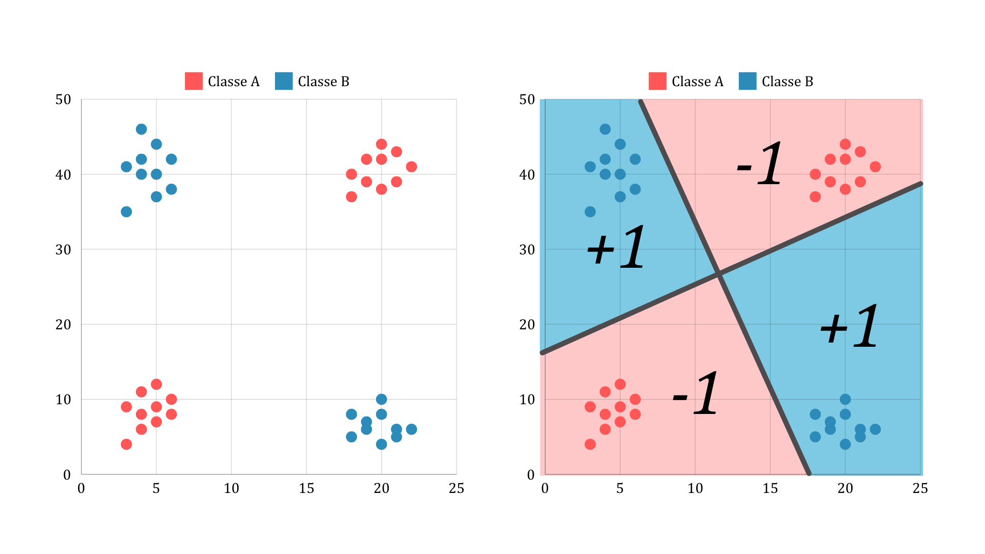
A single perceptron like the one we saw before cannot classify these points. However, we can combine the outputs of two perceptrons to build our classifier. Consider a perceptron that implements the classification shown in figure A, and another that implements the classification shown in figure B.

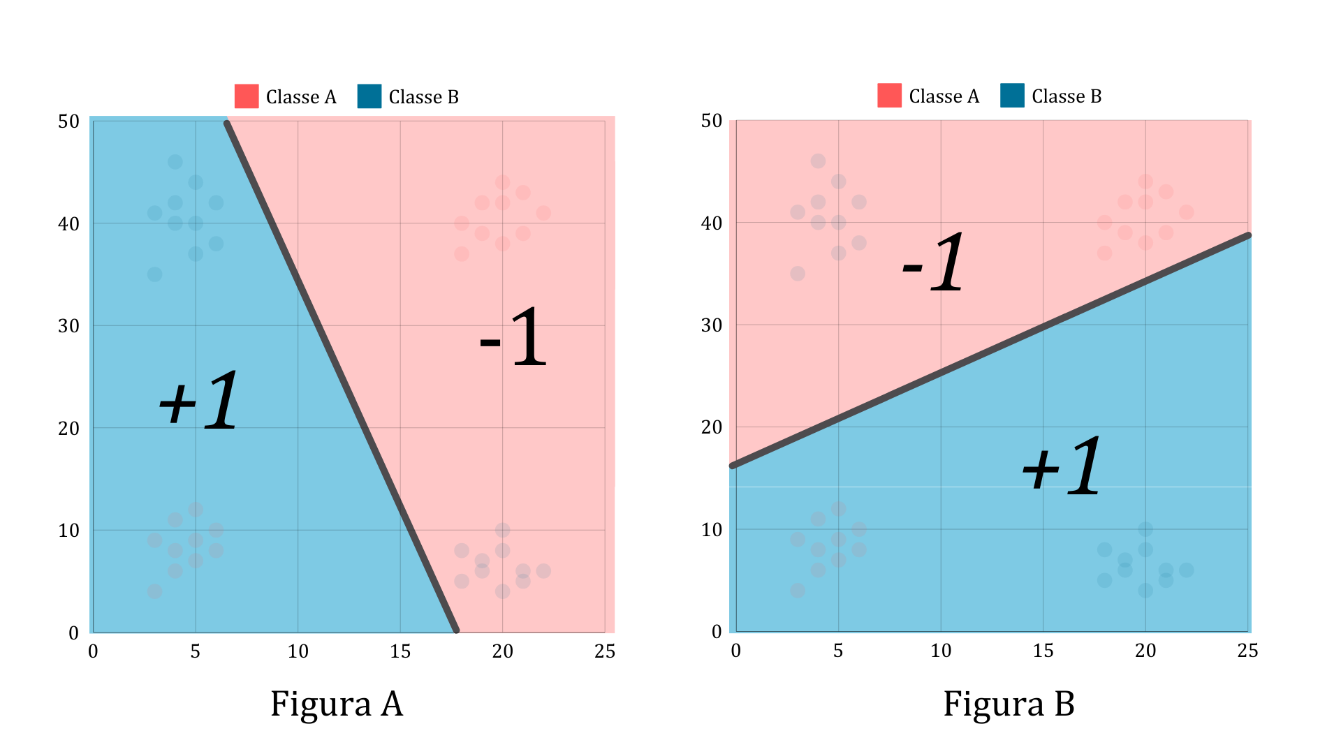
If we combine the results of these two perceptrons using a logical XOR, we get the correct classification for the problem we initially had. The good news is that the logical AND and the logical OR can also be built using perceptrons! So, a combination of perceptrons can give us the classifier we want.

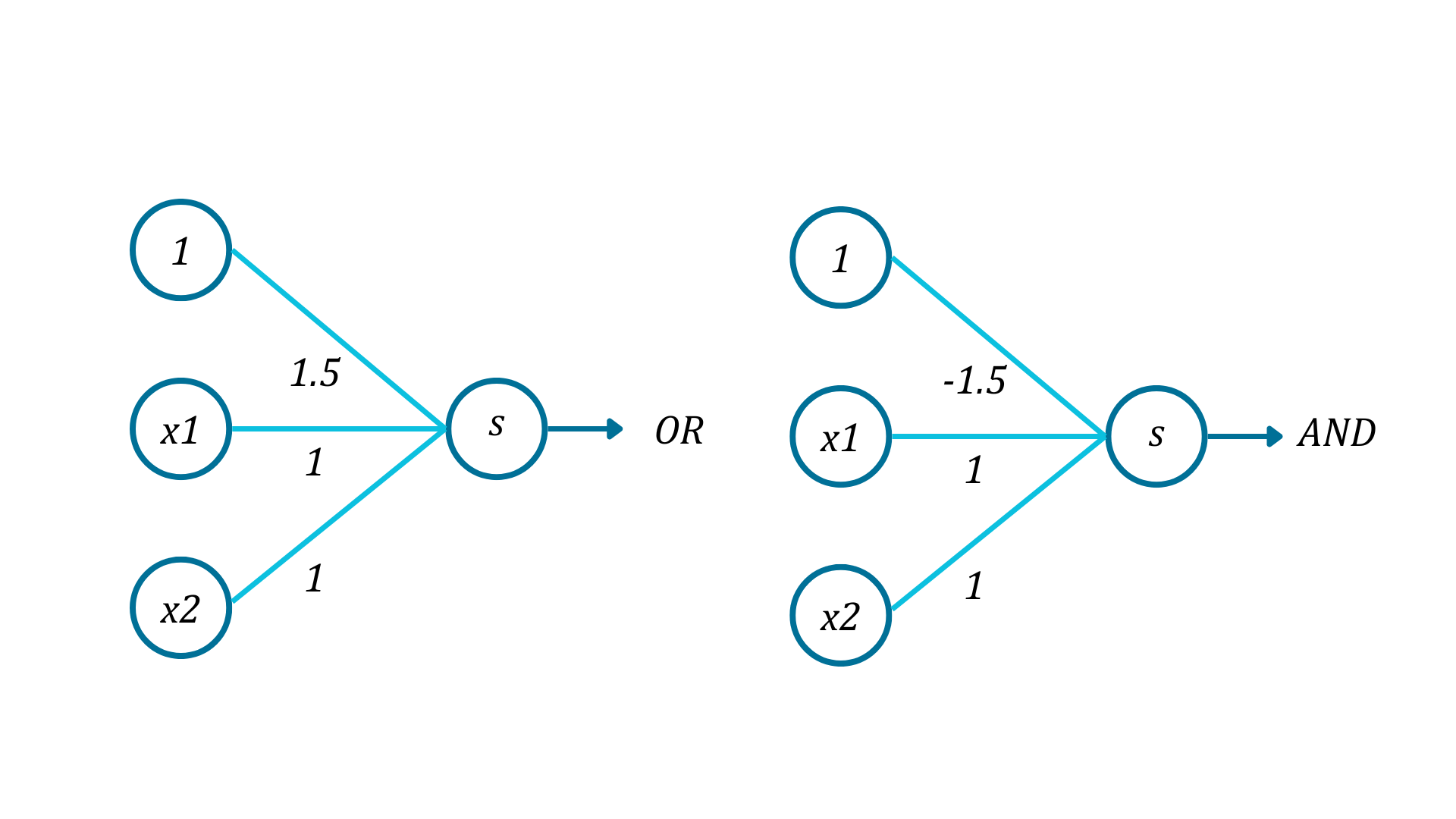
Perceptrons that implement logical OR and AND: $$OR(x_1, x_2) = \text{sign}(x_1 + x_2 + 1.5) $$ $$AND(x_1, x_2) = \text{sign}(x_1 + x_2 - 1.5) $$

Combining Perceptrons - Multi-layer Perceptron

To better understand perceptrons and their combinations, we are going to use a graphical representation of perceptrons as nodes. Here are the perceptrons for the logical AND and OR. The numbers on the lines represent the multiplication of the inputs to the nodes by those values. Everything that goes into a node is summed up, and the S in the final node represents the sign function.

The XOR function that we want to implement can be written as a combination of ANDs and ORs. $$XOR(x_1, x_2) = OR(AND(x_1, \bar x_2), AND(\bar x_1, x_2))$$ We can implement this by using the output of one perceptron as the input for another. Here is the combination we get:

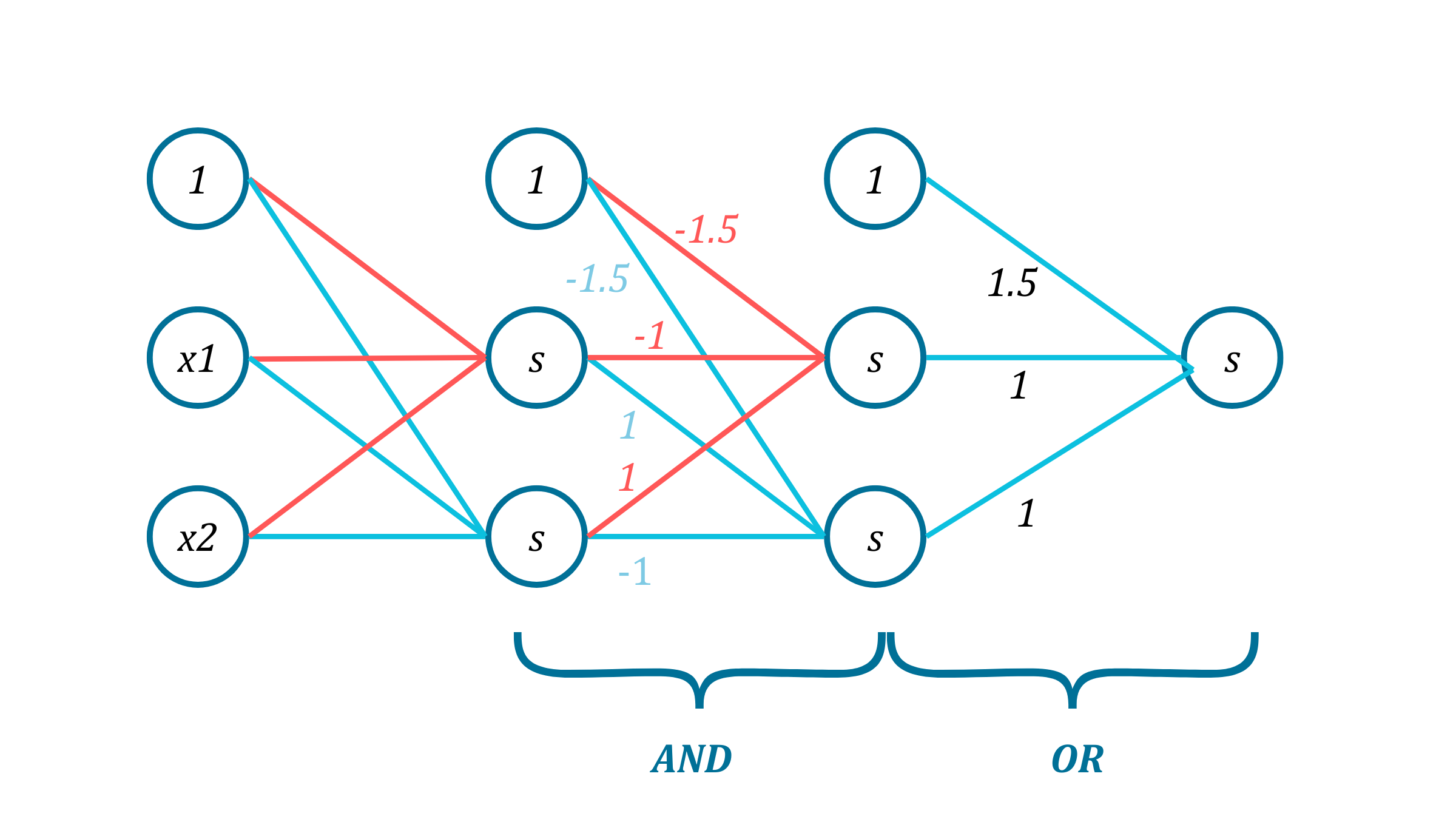
Notice that this combination of perceptrons forms multiple layers, hence the name Multi-layer perceptron (MLP). The first and the last layers are for input and output respectively. And the layers in the middle are called hidden layers. The idea of grouping perceptrons is the idea behind neural networs. Theses groupings of small units allow us to model all kinds of smooth functions. If we can decompose a function as a combination of ANDs and ORs of perceptrons, it can be modeled by an MLP. The picture below might give a sense of that. We can add layers and nodes to fit more complex functions. (However, one must do it with care in order not to loose generalization and end up with overfitting.) Once we fix the number of layers and nodes, we use the dataset to fit the function.

Fitting the data to an MLP, however, may lead to a hard combinatorial optimization problem! In the next post we will introduce Neural Networks and see how this is done with forward propagation and backward propagation.